| 2021 super output area - middle layer | Total | 1. Managers, directors and senior officials | 2. Professional occupations | 3. Associate professional and technical occupations | 4. Administrative and secretarial occupations | 5. Skilled trades occupations | 6. Caring, leisure and other service occupations | 7. Sales and customer service occupations | 8. Process, plant and machine operatives | 9. Elementary occupations | Tenure of household |
|---|---|---|---|---|---|---|---|---|---|---|---|
| E02006933 : Liverpool 061 | 401 | 74 | 152 | 69 | 29 | 16 | 14 | 16 | 14 | 17 | Owns with a mortgage or loan or shared ownership |
| E02003876 : Cheshire West and Chester 012 | 748 | 114 | 160 | 129 | 57 | 103 | 32 | 26 | 78 | 49 | Owns with a mortgage or loan or shared ownership |
| E02003211 : Bournemouth, Christchurch and Poole 048 | 703 | 284 | 182 | 106 | 33 | 34 | 22 | 13 | 15 | 14 | Owns with a mortgage or loan or shared ownership |
| E02003705 : Buckinghamshire 042 | 323 | 42 | 66 | 45 | 25 | 39 | 17 | 20 | 40 | 29 | Owns outright |
| W02000125 : Ceredigion 010 | 301 | 29 | 50 | 27 | 20 | 62 | 39 | 14 | 23 | 37 | Private rented or lives rent free |
| E02001615 : Sheffield 005 | 982 | 180 | 279 | 138 | 74 | 158 | 31 | 31 | 55 | 36 | Owns with a mortgage or loan or shared ownership |
Introduction
Private renting has expanded across the UK, yet the propensity to rent varies widely across occupations and life stages. This study quantifies how occupation and age relate to private rentership using 2021 ONS Census cross‑tabulations at the MSOA (neighbourhood‑scale) level. Housing tenure for household reference persons is linked to occupational categories and augmented with local authority identifiers to capture geographic context.
The analysis addresses three questions:
- Do higher‑skilled occupations rent less than lower‑skilled groups after accounting for age composition?
- How does rentership vary across life stages (age) ?
- To what extent do local authorities and neighbourhoods moderate these relationships?
The study is descriptive and subject to measurement constraints: age composition is observed for all workers rather than HRPs, and the focus is on full‑time employment. Despite these limitations, the findings provide a transparent baseline on how occupational structure and local context shape rental demand and motivate future work with richer microdata and dynamic market indicators.
Data
We use 2021 ONS Census data (via the Nomis API) that cross‑tabulates housing tenure and occupation at the MSOA level (“RM140: Tenure by Occupation - Household Reference Persons” 2023).
MSOAs (Middle Layer Super Output Areas) are neighborhood‑sized geographies. Counts refer to the household reference person (HRP) the person who represents the household, so each household is linked to a single occupation.
These are different from the counts of all workers (used in occupation‑by‑age data introduced later in the study), because a household can contain more than one person in full‑time work but only one HRP.
Additional information
Local authority for each MSOA in original dataset is added, to account for rental patterns that may be present at local area levels. Being in the same Local authority may affect neighbouring MSOAs introducing correlations in their data.
It may be the case that age has a confounding effect on Rentership via Occupation. Professional and Managers may likely be older than for e.g. Associates and this may mean that they were able to purchase a house earlier in their careers/life and now represent a smaller proportion of rental cohort.
Adjusting for age gives an apples-to-apples comparison of rentership preference among people pursuing different occupations but are in boradly same phases of their life.
The adjustment can be made (ideally) by including the counts of full-time employed HRPs in an MSOA engaged in a particular profession.
We have cross tabulated data (“RM102: Occupation by Age - Residents in Employment” 2023) for counts of usual residents aged 16 years and over in employment the week before the census per occupation, falling in one of the following age bands:
- aged 15 years and under
- aged 16 to 24 years
- aged 25 to 34 years
- aged 35 to 49 years
- aged 50 to 64 years
- aged 65 years and over
Note:
Using this data gives an inexact adjustment since this data is available for all residents aged 16 years and over in employment rather than just HRP (which is the unit of measurement in tenure data). This means that an HRP could be a singular older person, whereas the counts in age dataset include other members of the household which are possibly younger, creating a slight disconnect between the 2 datasets.
It is neverthless instructive to use this data as the downsides due to excluding this information outweigh downsided due to (incorrectly) including it.
Since, the interest lies in proportion of rentership for each occupation, per occupation totals for each MSOA are added to the dataset, setting us up for a Binomial counts of Success-Failures type of model.
Filter
Current data only includes measurements from household reference persons (HRP) in full time employment a week before census.
London is also filtered out as it is a very different rental market compared to the rest of UK and may skew results when mixed with other regions.
Note:
- ONS rental tenure data includes a large proportion (~34%) of people not under full time employment(“Annex Table 1.5: Employment Status by Tenure,2021-22” 2023) (filtered out in current analysis)
- part-time work (~11% includes furloughed)
- retired (~7%)
- unemployed (~4%)
- full-time education (~4%)
- other inactive (~8%)
- The private rented sector houses the highest proportion of non-UK nationals (74% of HRPs in the private rented sector are from the UK, compared to 92% of social renters and 96% of owner occupiers) (“English Housing Survey 2021 to 2022: Private Rented Sector” 2023)
| msoa | tenure | occupation | counts_of_hrp | occupation_total | aged 15 years and under | aged 16 to 24 years | aged 25 to 34 years | aged 35 to 49 years | aged 50 to 64 years | aged 65 years and over | all_ages_total | region | lad_name |
|---|---|---|---|---|---|---|---|---|---|---|---|---|---|
| e02003738 | private rented or lives rent free | 4. administrative and secretarial occupations | 17 | 128 | 0 | 25 | 49 | 98 | 121 | 21 | 314 | e12000006 | east cambridgeshire |
| e02004479 | private rented or lives rent free | 3. associate professional and technical occupations | 44 | 320 | 0 | 86 | 171 | 201 | 157 | 16 | 631 | e12000006 | castle point |
| e02001840 | private rented or lives rent free | 2. professional occupations | 59 | 305 | 0 | 28 | 162 | 194 | 84 | 5 | 473 | e12000005 | birmingham |
| e02005068 | private rented or lives rent free | 7. sales and customer service occupations | 17 | 68 | 0 | 53 | 63 | 33 | 59 | 11 | 219 | e12000008 | maidstone |
| e02005669 | private rented or lives rent free | 1. managers, directors and senior officials | 24 | 355 | 0 | 11 | 58 | 207 | 221 | 29 | 526 | e12000004 | west northamptonshire |
| e02003597 | private rented or lives rent free | 3. associate professional and technical occupations | 33 | 150 | 0 | 14 | 40 | 82 | 106 | 19 | 261 | e12000008 | isle of wight |
Subsample
Since, the dataset is very well compiled but is large, we can work with reduced dataset and infer large scale effects from it. This reduction will allow speeding up the analysis and experimentation.
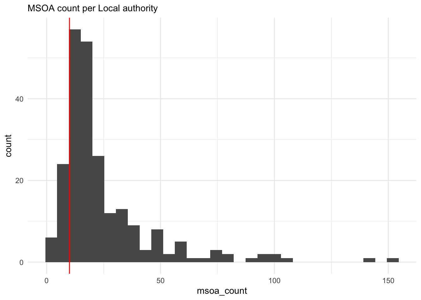
We can see that majority of Local authorities have 10-15 MSOAs. To get a balanced representation, we chose to sample 10 MSOA from each Local authority. This will likely also ensure robust estimation of any random effects.
The subsampling process does the following:
- Sample all local authorities from 8 UK wide regions (e.g. West midlands, East of England etc.) but excluding London region (since market behaviour may not generalise to other regions and create issues when data is mixed with others, due to very high counts)
- Within each of the local authorities sample 10 MSOAs at random
- Get all the data in the sampled MSOAs
The above procedure is deliberate in that it results in balanced data among Local authorities to avoid issues with inference.
It goes without saying that this step means that Local Authorities and MSOAs need to be treated as random effects down the line (with appropriate heirarchy).
The procedure ensures sufficient counts of Local Authorities and MSOAs to be able to reliably capture these random effects.
| rows | distinct_tenure | distinct_occupation | max_hrp_counts | min_hrp_counts | median_hrp_counts | distinct_lad | distinct_msoa |
|---|---|---|---|---|---|---|---|
| 20124 | 1 | 9 | 788 | 0 | 40 | 234 | 2236 |
EDA
At the level of MSOA the proportion of rentership can appear quite chaotic and noisy.
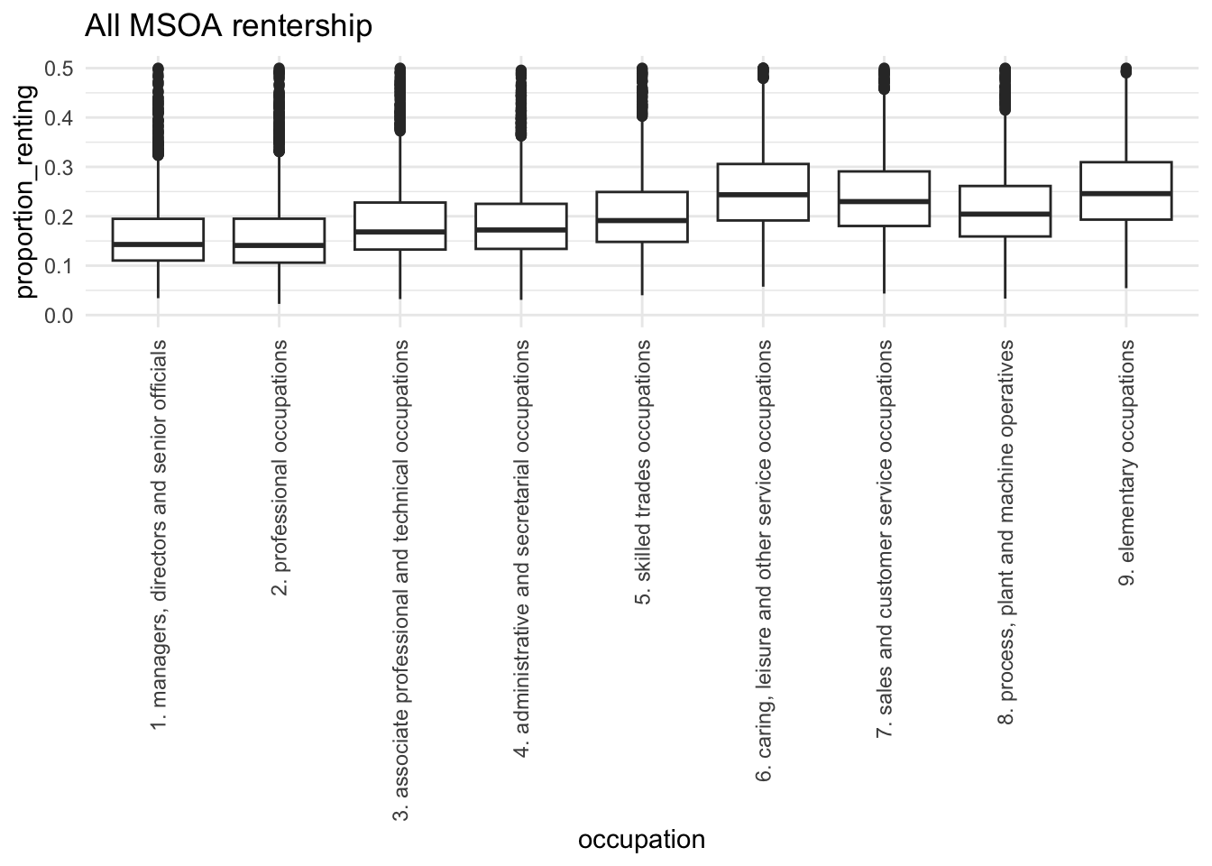
Aggregated data shows clear differences in renting by occupation. Highly skilled and professional workers rent less, likely because they can more easily afford to buy.
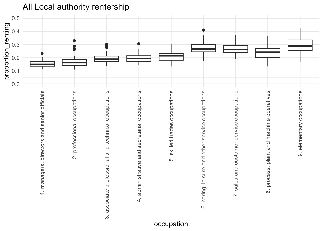
The observation holds and patterns become more clear when the data is aggregated at Local authority level. This means that a heirarchical consideration of geographies could be a sensible inclusion in the model.
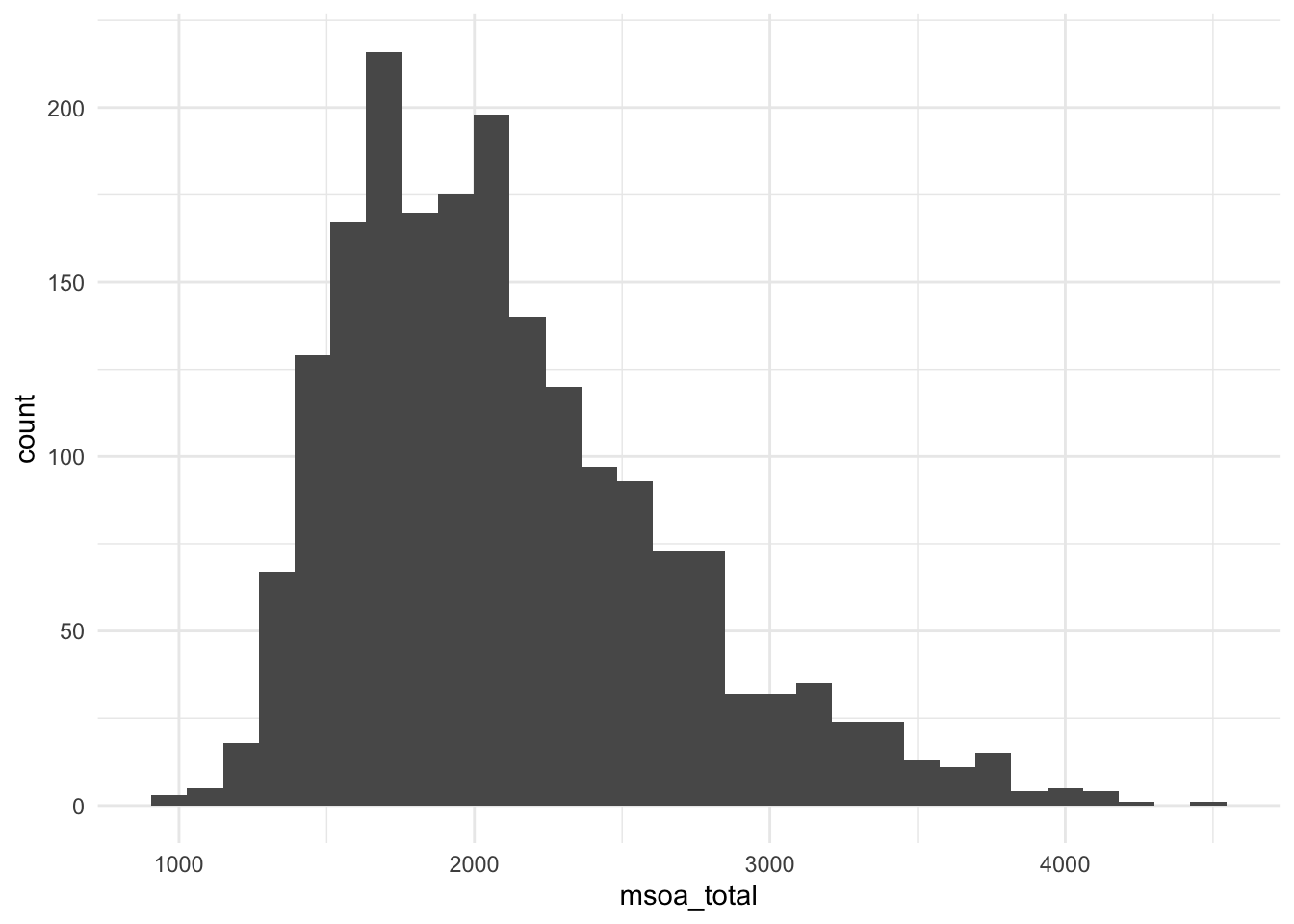
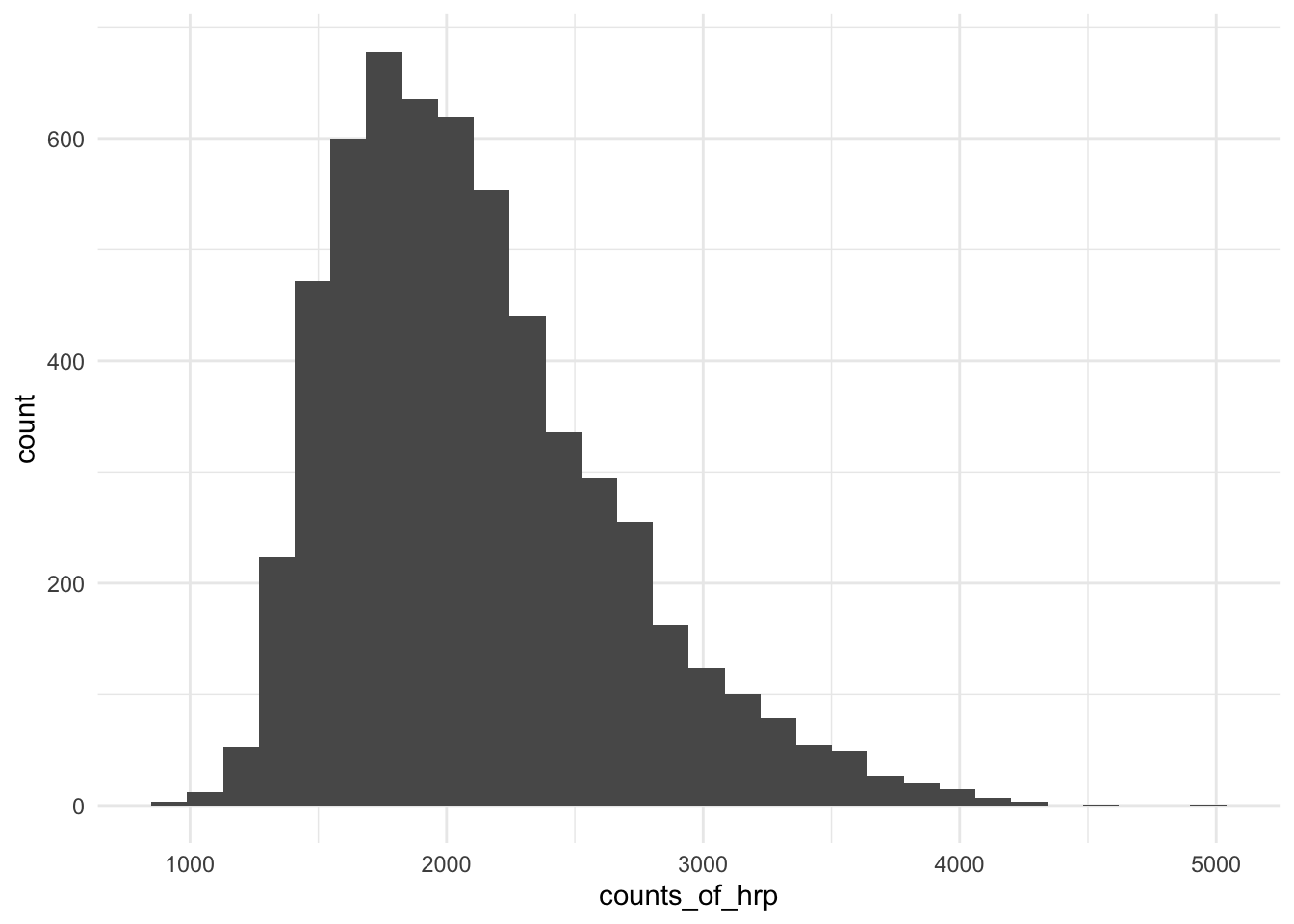
There is a slightly long tail of working population per msoa.
Looking at the msoa where the greatest proportion of working population is renting, a few key dense local authority areas are highlighted
| msoa | lad_name | counts_of_hrp | aggregate_proportion_renting |
|---|---|---|---|
| e02005029 | dartford | 4969 | 0.262 |
| e02004650 | tewkesbury | 4484 | 0.224 |
| e02004681 | basingstoke and deane | 4298 | 0.185 |
| e02005683 | west northamptonshire | 4266 | 0.168 |
| e02005614 | north northamptonshire | 4208 | 0.221 |
| e02004595 | uttlesford | 4175 | 0.156 |
| e02003643 | central bedfordshire | 4169 | 0.166 |
| e02005455 | north kesteven | 4147 | 0.182 |
| e02005924 | cherwell | 4146 | 0.485 |
| e02006270 | mid suffolk | 4093 | 0.266 |
The age distribution of working population varies significantly across occupations.
It is interesting to note that some occupations are over represented among older age groups (e.g. Managers and Professionals), whereas others are more evenly spread (e.g. Elementary operations).
Since, age data has a long tailed distribution, log scaling is used to better scale it and also make its interpretation in the model more intuitive.
Analysis
Baseline Model: Fixed effects without location information
We refer to data at MSOA level for modelling. For the baseline model, MSOA variable is excluded and Elementary occupations are treated as a reference category for Occupation variable. aged 15 years and under variable is dropped as it is irrelevant for this study. It is immediately obvious that occupation has significant association with proportion of people renting.
Analysis of Deviance Table
Model: binomial, link: logit
Response: cbind(renting_total, occupation_total - renting_total)
Terms added sequentially (first to last)
Df Deviance Resid. Df Resid. Dev Pr(>Chi)
NULL 20123 341677
occupation 8 58729 20115 282948 < 2.2e-16 ***
log(age_16_24 + 1) 1 20639 20114 262308 < 2.2e-16 ***
log(age_25_34 + 1) 1 11520 20113 250788 < 2.2e-16 ***
log(age_35_49 + 1) 1 28124 20112 222664 < 2.2e-16 ***
log(age_50_64 + 1) 1 19545 20111 203119 < 2.2e-16 ***
log(age_over_65 + 1) 1 3530 20110 199589 < 2.2e-16 ***
occupation:log(age_16_24 + 1) 8 6347 20102 193241 < 2.2e-16 ***
occupation:log(age_25_34 + 1) 8 1222 20094 192020 < 2.2e-16 ***
occupation:log(age_35_49 + 1) 8 1383 20086 190637 < 2.2e-16 ***
occupation:log(age_50_64 + 1) 8 3627 20078 187010 < 2.2e-16 ***
occupation:log(age_over_65 + 1) 8 2519 20070 184492 < 2.2e-16 ***
---
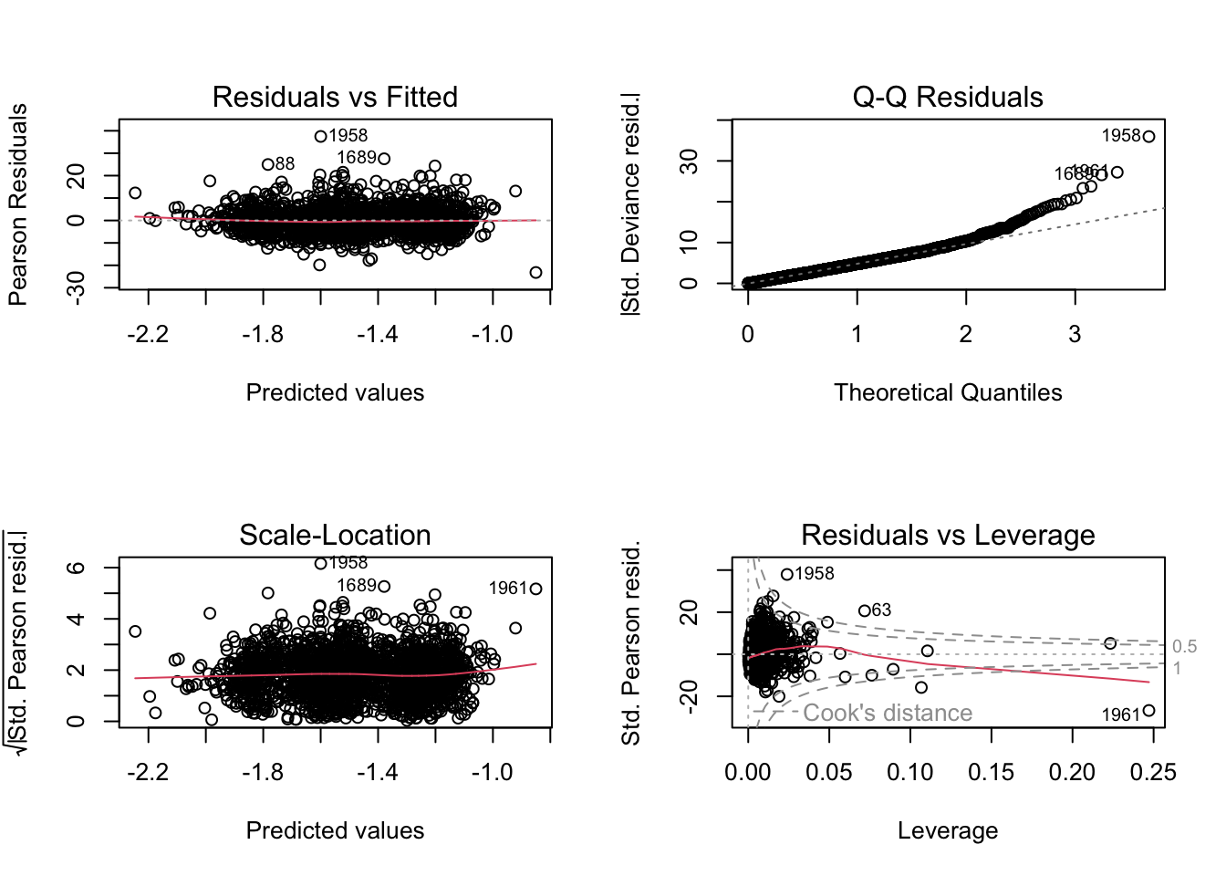
Signif. codes: 0 '***' 0.001 '**' 0.01 '*' 0.05 '.' 0.1 ' ' 1The Scale-location diagnostics and QQ-Residuals suggest the dispersion is much higher than expected. This is also confirmed by the dispersion parameter, 9.33
High residual points can be investigated to identify some issues.
Primarily, these seem to areas in the city centers where rentership is much higher than what the model predicts and can be seen on the map too.
| msoa | lad_name | occupation | age_16_24 | age_25_34 | age_35_49 | age_50_64 | age_over_65 | renting_total | occupation_total | .resid | actual_renting_proportion | predicted_proportion |
|---|---|---|---|---|---|---|---|---|---|---|---|---|
| e02001432 | sefton | 9. elementary occupations | 149 | 195 | 238 | 197 | 34 | 382 | 477 | 18.31027 | 0.80 | 0.39 |
| e02003293 | southend-on-sea | 6. caring, leisure and other service occupations | 71 | 158 | 247 | 197 | 31 | 307 | 436 | 17.71392 | 0.70 | 0.29 |
| e02003516 | brighton and hove | 2. professional occupations | 97 | 590 | 531 | 289 | 36 | 662 | 1071 | 17.47028 | 0.62 | 0.36 |
| e02003430 | windsor and maidenhead | 2. professional occupations | 36 | 208 | 347 | 290 | 30 | 242 | 506 | 17.17201 | 0.48 | 0.15 |
| e02004365 | eastbourne | 6. caring, leisure and other service occupations | 108 | 203 | 287 | 185 | 21 | 326 | 442 | 17.08044 | 0.74 | 0.34 |
| e02003514 | brighton and hove | 3. associate professional and technical occupations | 95 | 434 | 389 | 179 | 19 | 447 | 728 | 16.96523 | 0.61 | 0.31 |
| e02003293 | southend-on-sea | 5. skilled trades occupations | 55 | 131 | 214 | 151 | 16 | 251 | 386 | 16.82279 | 0.65 | 0.24 |
| e02003226 | swindon | 2. professional occupations | 44 | 240 | 262 | 73 | 4 | 276 | 425 | 16.41195 | 0.65 | 0.27 |
| e02004365 | eastbourne | 5. skilled trades occupations | 48 | 104 | 155 | 113 | 7 | 203 | 297 | 15.97221 | 0.68 | 0.24 |
| e02004378 | hastings | 3. associate professional and technical occupations | 24 | 137 | 238 | 198 | 36 | 213 | 455 | 15.84288 | 0.47 | 0.15 |
Overall it appears that including location information in the model is necessary to account for area-specific rentership patterns.
Introducing location context in the model
Each MSOA can have its own level of rentership that needs to be accounted for (and town centers can be very different from suburbs).
This is an opportunity for us to introduce location information (LAD and MSOA) in the model. We shall be mindful of the fact that the MSOA are randomly chosen and that MSOA are nested inside LAD.
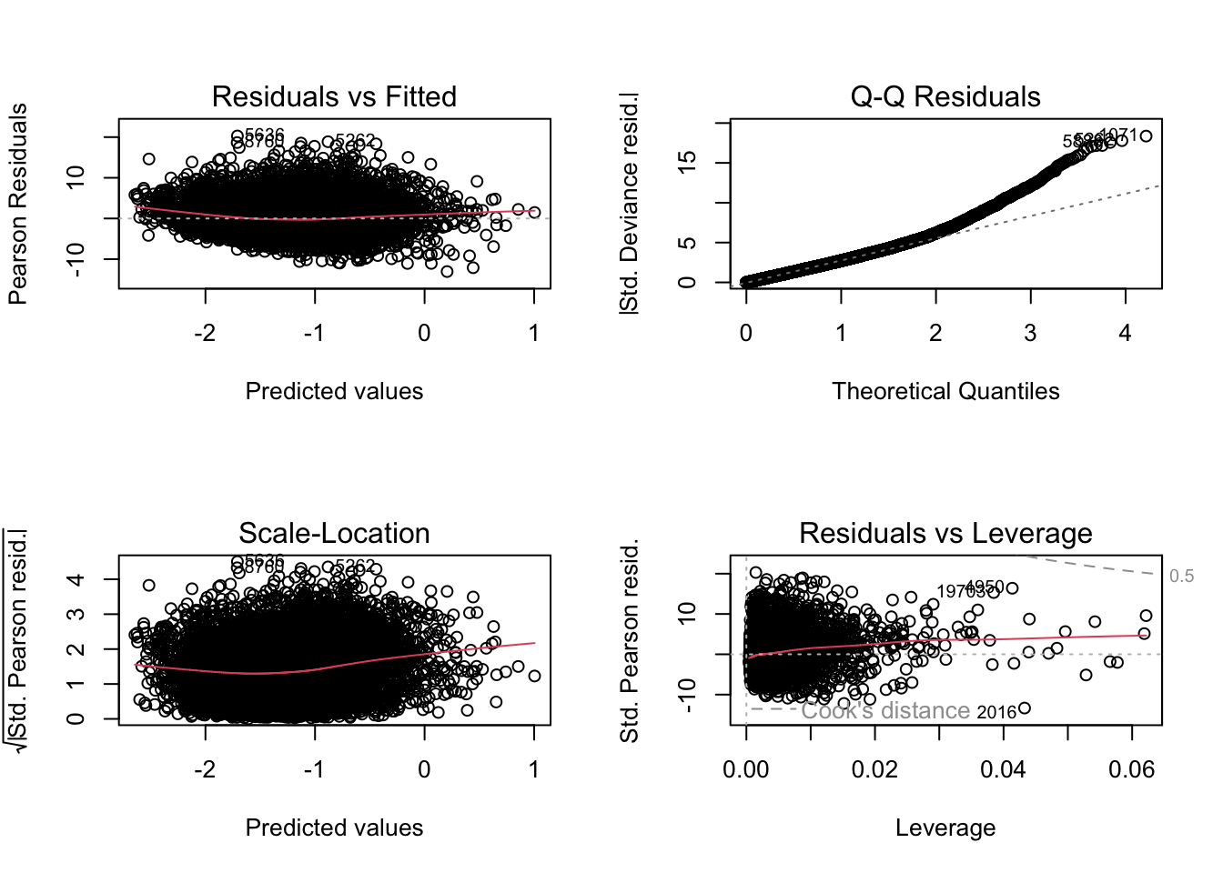
Model evaluation
Diagnostics have improved and residuals are smaller than before, so the addition of MSOAs in model is worthwhile.
Error by occupation
The model captures renting behaviour across different occupations reasonably well and does not seem to have biased results for any.
An avenue for improvement can be with more information relevant to Elementary occupations and Professional occupations where the model seems to make large errors compared to others.
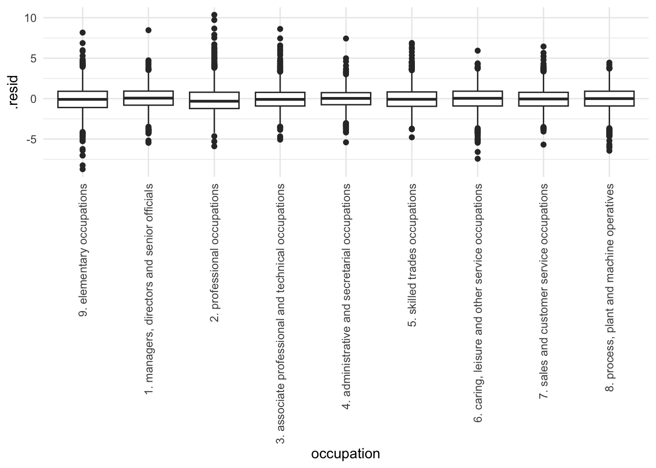
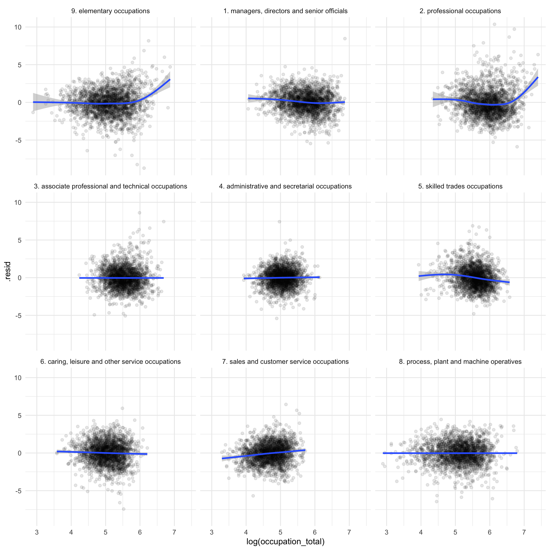
The model is robust to how many people are engaged in particular occupations. It seems to make similar magnitudes of errors and on average is unbiased. For e.g. the accuracy is coparalble at a location fewer occupants are Managers vs a location where several occupants are Managers.
Comparison
Comparing predictions from the 2 models on the list of worse cases highlighted earlier, there again seems to be an improvement.
| msoa | lad_name | occupation | renting_total | occupation_total | actual_renting_proportion | predicted_proportion_base | predicted_proportion_glmer |
|---|---|---|---|---|---|---|---|
| e02001432 | sefton | 9. elementary occupations | 382 | 477 | 0.80 | 0.39 | 0.72 |
| e02003293 | southend-on-sea | 6. caring, leisure and other service occupations | 307 | 436 | 0.70 | 0.29 | 0.63 |
| e02003516 | brighton and hove | 2. professional occupations | 662 | 1071 | 0.62 | 0.36 | 0.61 |
| e02003430 | windsor and maidenhead | 2. professional occupations | 242 | 506 | 0.48 | 0.15 | 0.35 |
| e02004365 | eastbourne | 6. caring, leisure and other service occupations | 326 | 442 | 0.74 | 0.34 | 0.70 |
| e02003514 | brighton and hove | 3. associate professional and technical occupations | 447 | 728 | 0.61 | 0.31 | 0.59 |
| e02003293 | southend-on-sea | 5. skilled trades occupations | 251 | 386 | 0.65 | 0.24 | 0.58 |
| e02003226 | swindon | 2. professional occupations | 276 | 425 | 0.65 | 0.27 | 0.53 |
| e02004365 | eastbourne | 5. skilled trades occupations | 203 | 297 | 0.68 | 0.24 | 0.63 |
| e02004378 | hastings | 3. associate professional and technical occupations | 213 | 455 | 0.47 | 0.15 | 0.49 |
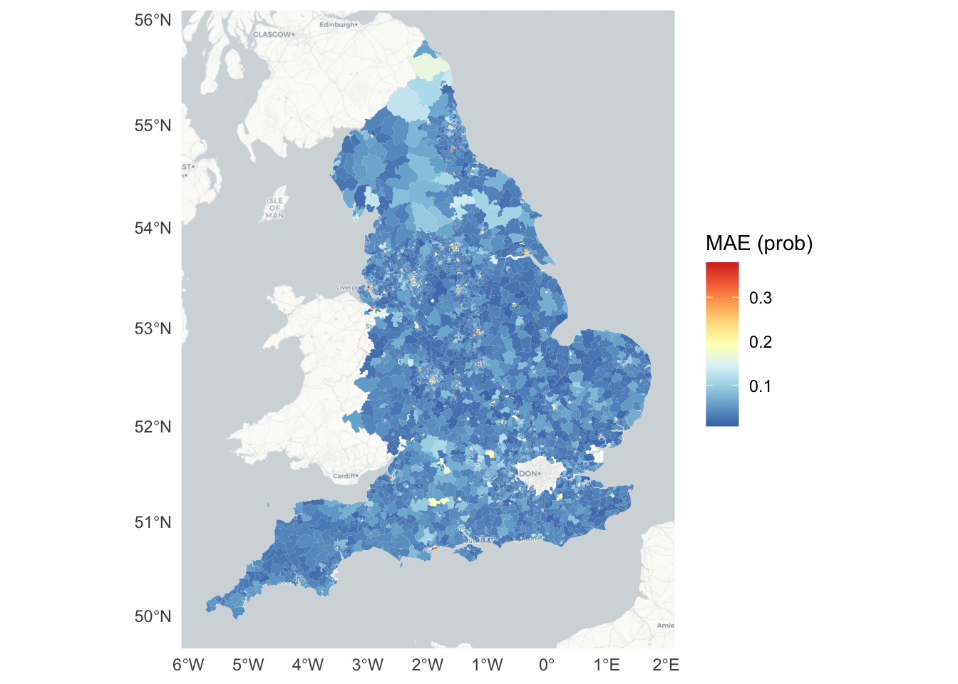
Error behaviour spatially
The error in predicted probability of rentership is small for several MSOAs, even though a small subset was used in modelling. This is another good reason to retain the current model.
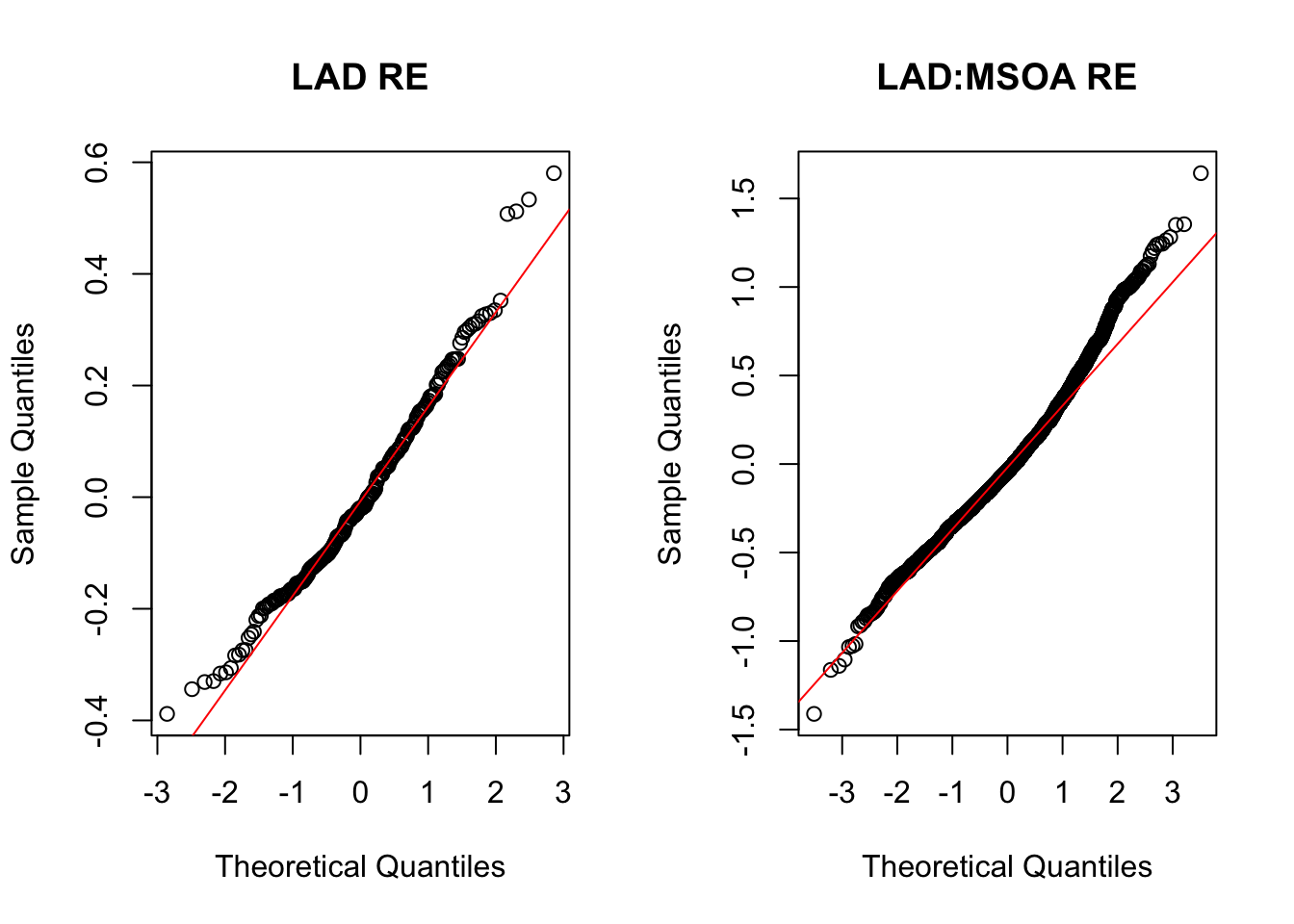
Random effects and dispersion
Random effects of LAD appear reasonably normally distributed.
MSOA nested inside LAD are slighly more dispersed and have longer tails, but it doesn’t seem too problematic to affect reliability of the model.
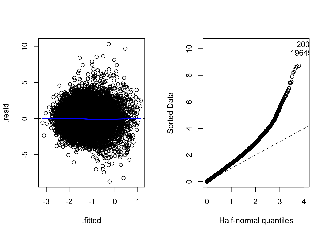
Before moving to inference using this model, it is important to check how it fits. ChiSq GoF test suggests p-value 0, which indicates that there is still quite a lot of variance in data that isn’t explained by the current model.
The dispersion parameter is 2.08. This indicates that there is some degree of overdispersion. It is likely a result of not including more factors affecting rentership (e.g. presence of employers, type of location, commute etc.) and using a simplistic model. The overdispersion is largely relevant for standard errors, but fixed effects which are our quantity of interest should be unchanged. Inference will likely be worse but with such a simplistic model we do not expect significant impact. We shall retain the current model as it is since it provides useful insights as we shall see in the following sections.
Interpretation and application
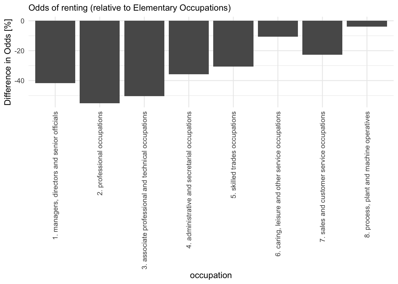
Occupation effect
Looking at the coefficients of Occupation types, since Elementary Occupations was reference class, the odds for any Occupation are relative to it.
In general any Occupation category is less likely to rent compared to Elementary Occupations, in particular Professionals are nearly 55% less likely (0.44x) to rent.
There is intuitive sense to the effects as higher paid occupations are less likely to rent, except interestingly that unlike observations in raw data, Managers are not the least likely renters when age is taken into account.
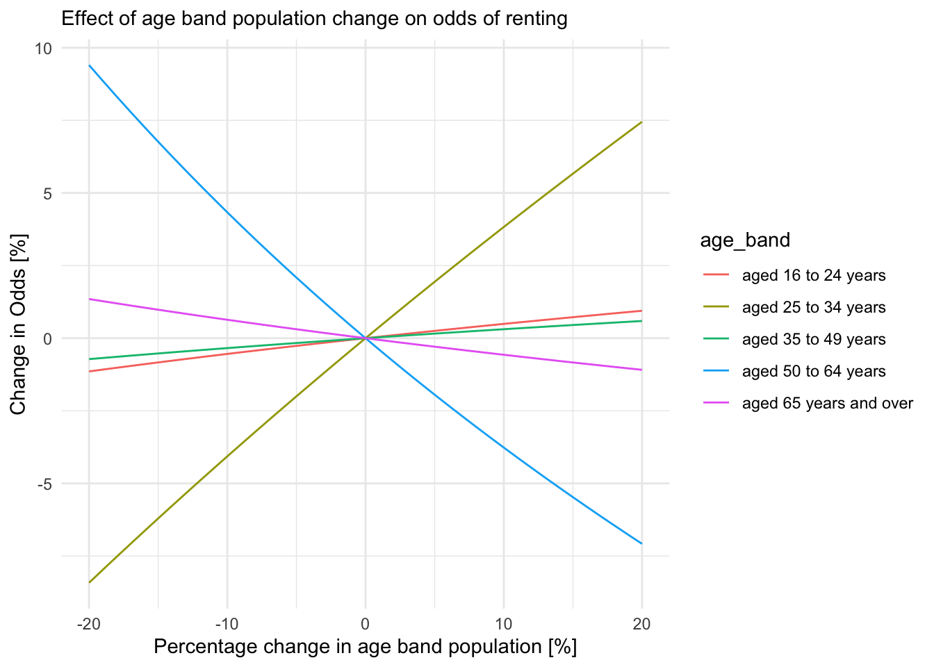
Age effect
Age plays a key role in likelihood of renting too. Rentership is highly sensitive to population in 25-34 year age bracket. With a 10% increase in population in that age bracket, odds increase by approx 3.8%
Conclusion
This analysis provides descriptive evidence that who rents, and where, is shaped by occupation and age. Across UK MSOAs (excluding London), higher‑skilled groups—especially professionals—are consistently less likely to rent than lower‑skilled groups. Rentership peaks among 25–34 year olds, and remains sensitive to the age mix in local working populations. Introducing local authority and neighbourhood random effects improves fit and reveals meaningful spatial variation: town centres and dense urban MSOAs tend to have higher rentership than suburban areas, even after adjusting for occupation and age.
The models are simple and intentionally transparent. While they capture core patterns, residual variance and mild overdispersion indicate omitted local factors (e.g., price levels, employer presence, transport access) still matter. Results should be interpreted as associations, not causal effects.
Several limitations are important. Age‑by‑occupation counts refer to all workers rather than household reference persons, creating a measurement disconnect with tenure data. London is excluded, so findings do not generalise to its market. The analysis is cross‑sectional and does not track transitions into or out of renting.
Despite these caveats, the evidence suggests rental demand is highest where younger workers are concentrated and falls with occupational skill. For planning and housing supply, this points to tailoring new rental provision toward places with strong 25–34 cohorts and occupations more likely to rent.
References
“Annex Table 1.5: Employment Status by Tenure,2021-22.” 2023. Department for Levelling Up, Housing; Communities. https://assets.publishing.service.gov.uk/media/64ad65e48bc29f000d2cca7f/EHS_21-22_PRS_Ch_1_Annex_Tables.ods.
“English Housing Survey 2021 to 2022: Private Rented Sector.” 2023, July. https://www.gov.uk/government/statistics/english-housing-survey-2021-to-2022-private-rented-sector/english-housing-survey-2021-to-2022-private-rented-sector.
“RM102: Occupation by Age - Residents in Employment.” 2023. Office for National Statistics. https://www.ons.gov.uk/datasets/RM102/editions/2021/versions/3.
“RM140: Tenure by Occupation - Household Reference Persons.” 2023. Office for National Statistics. https://www.ons.gov.uk/datasets/RM140/editions/2021/versions/2.