| user_id | date | registration_date |
|---|---|---|
| d8c465ab-e9fd-5edd-9e4e-c77094700cb5 | 2020-10-01 | 2020-08-25 |
| 269b7f13-a509-5174-85cb-95a8f7b932e8 | 2020-10-01 | 2020-08-25 |
| bfeac474-5b66-566f-8654-262bb79c873e | 2020-10-01 | 2020-05-31 |
| d32fcac5-122c-5463-8aea-01b39b9ad0bb | 2020-10-01 | 2020-09-30 |
| c1ece677-e643-5bb3-8701-f1c59a0bf4cd | 2020-10-01 | 2020-09-05 |
| ba6750c9-9b60-58dc-8d40-504e7375249e | 2020-10-01 | 2020-09-29 |
Introduction
Duolingo have been making waves with their customer success stories and strong (and growing) user base. They seem to be taking their metrics seriously and have done a great job explaining their approach to understanding user behaviour in this (Gustafson 2024).
In the current blog, I wanted to apply their methodology and use it for predicting future customer behaviours.
The problem statement driving this analysis is simple. Duolingo want to predict their future daily active users (DAU) with some control handles that they can manipulate to improve those numbers e.g. send reminders to at risk weekly active users or reward campaigns to at risk monthly active users.
They may be able to run (or have already run) experiments identifying the effects of these campaigns and reminder in terms of % of people that respond to the treatment and revert back to being daily active.
This allows them to efficiently allocate resources and maintain a healthy user base that eventually materialises into paying customers.
Methodology
First we shall model the process as a Markov chain to see how well the approach predicts future user counts.
Subsequently, to validate MC approach and rethink the problem setup in want of simplification, we shall look to model the time-series as a regression problem. We shall do this respecting the mechanics of transition and see how far this can get us in terms of analysing and controlling the process.
At day d (d = 1, 2, … ) of a user’s lifetime, the user can be in one of the following 7 (mutually-exclusive) states:
- new : learners who are experiencing Duolingo for the first time ever
- current : learners active today, who were also active in the past week
- reactivated : learners active today, who were also active in the past month (but not the past week)
- resurrected : learners active today, who were last active >30 days ago
- at_risk_wau (at risk weekly active users) : learners who have been active within the past week, but not today
- at_risk_mau (at risk monthly active users) : learners who were active within the past month, but not the past week
- dormant : learners who have been inactive for at least 30 days
A brief overview of how these states are related is below:
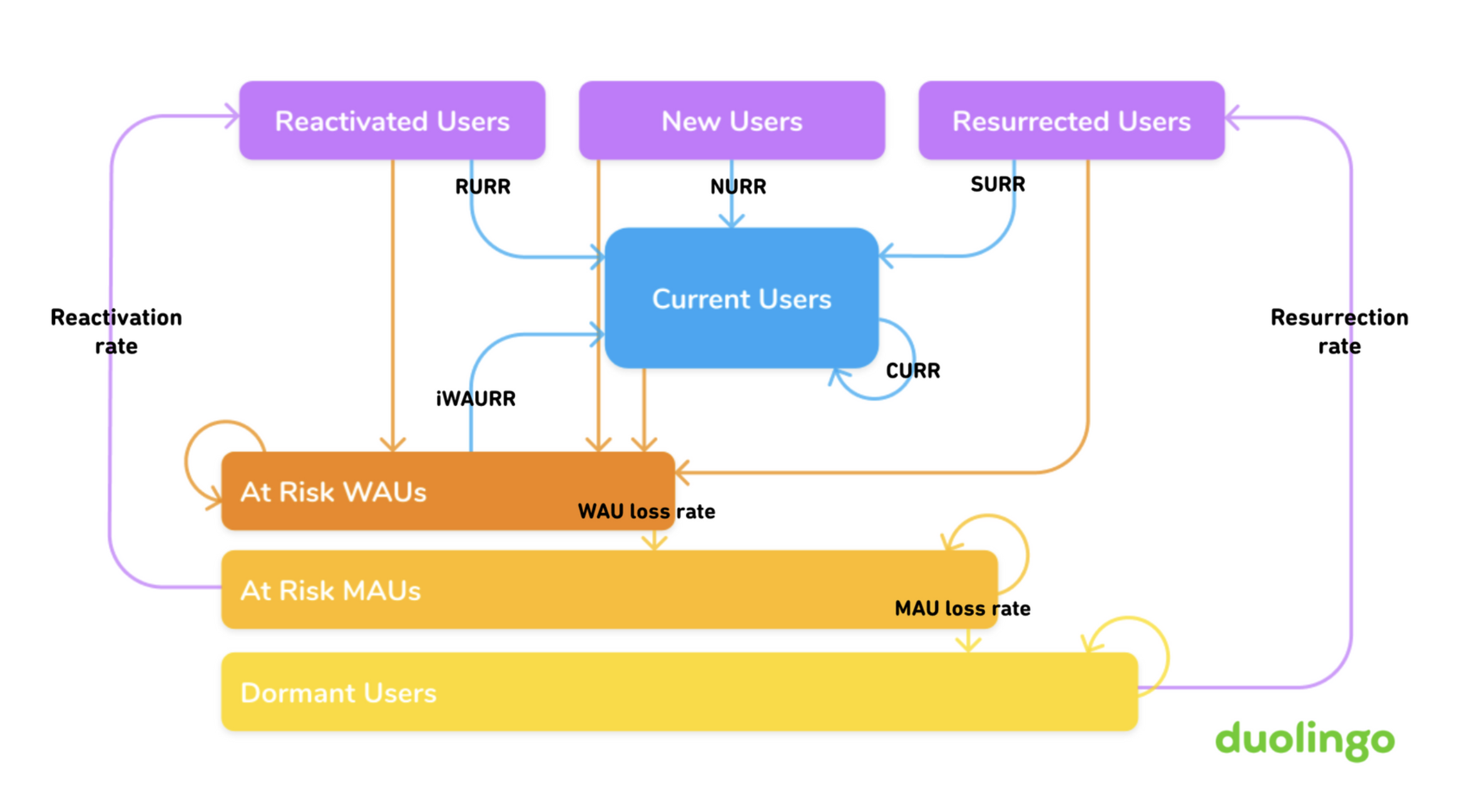
The transition acronyms are defined below:
- NURR : New User Retention Rate (The proportion of day 1 learners who return on day 2)
- CURR : Current User Retention Rate (This is not a 100%. Not all of current users stay active every day since people forget to complete a lesson, or have technical difficulties, or just want to take a break)
- RURR : Reactivated User Retention rate (The proportion of at_risk_mau who became active today)
- SURR : Resurrected User Retention rate (The proportion of dormant users who became active today)
- iWAURR : The proportion of at_risk_wau users who became active today
As is evident, these quantities (along with others) are what will become the elements of Transition matrix (M), that we discuss next.
In keeping with the definition chart above, the next step is to consider user behaviour as a Markov chain.
Let M be a transition matrix associated with this Markov process: m(i, j) = P(s_j | s_i) are the probabilities that a user moves to state s_j right after being at state s_i. The matrix M is learned from the historical data.
Assuming that user behavior is stationary (independent of time), the matrix M fully describes the states of all users in the future.
Suppose that the vector u_0 of length 7 contains the counts of users in certain states on a given day (say day 0). According to the Markov model, on the next day (day 1), we expect to have the following number of users (u_1) in respective states:
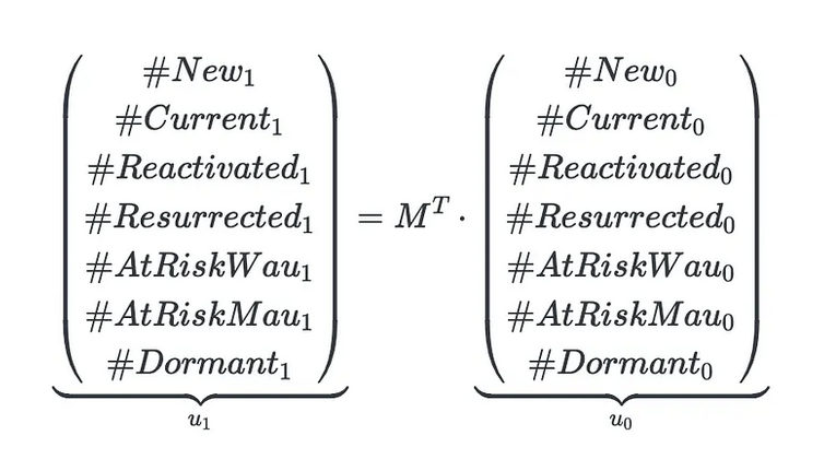
Applying this multiplication recursively, we can derive the number of users in any states on any arbitrary day t > 0 in the future (call this vector u_t).
Now, having u_t calculated, we can determine DAU, WAU and MAU values on day t:
- DAU_t = #New_t + #Current_t + #Reactivated_t + #Resurrected_t
- WAU_t = DAU_t + #AtRiskWau_t
- MAU_t = DAU_t + #AtRiskWau_t + #AtRiskMau_t
Finally, here’s the algorithm outline:
- For each prediction day t = 1, …, T, calculate the expected number of new users #New_1, …, #New_T.
- For each lifetime day of each user, assign one of the 7 states.
- Calculate the transition matrix M from the historical data.
- Calculate initial state counts u_0 corresponding to day t=0.
- Recursively calculate u_{t+1} = M^t * u_0.
- Calculate DAU, WAU, and MAU for each prediction day t = 1, …, T.
Data
We use a simulated dataset based on historical data of a SaaS app.
The data is available here and contains three columns: user_id, date, and registration_date.
Each record indicates a day when a user was active.
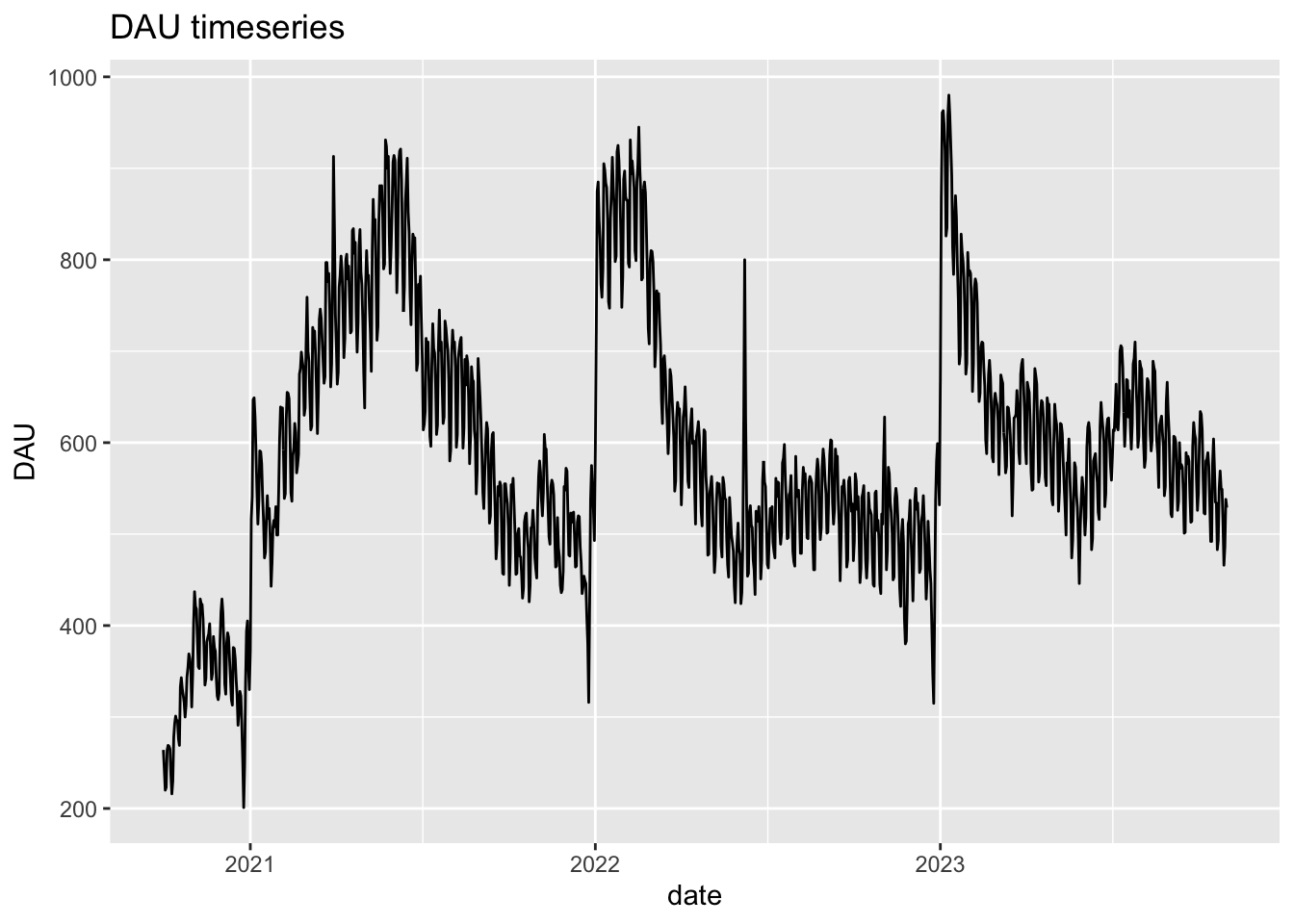
Total users: 51480Date range: 2020-10-01 to 2023-10-31This is how DAU timeseries looks
Model
Future new user count model
To even begin thinking about transitions on a future date, we first need to acknowledge the fact that new user counts will be a significant missing piece of information in the analysis.
To get around this limitation, we shall first build a new user count prediction model that need not be very accurate (since in a realistic setting new user counts can also be a parameter that can be changed).
The information on new users on any given date is inherent in registration_date in the data.
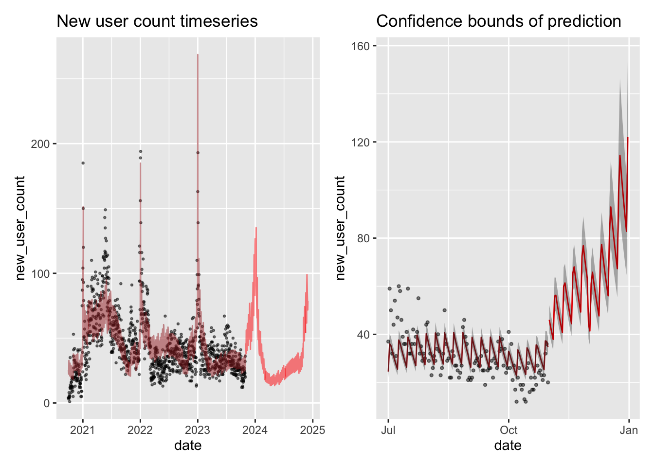
After some experimentation, the model setup to predict future counts of new users is as above.
The counts are assumed Poisson but with a higher variance than normal due to spikes in the data and hence a negative binomial model has been used.
It was imperative that we used a robust version of GLM to be able to get relatively constant variance of errors, that were being caused due to outliers in user count towards beginning of every year.
The model appears to be doing a satisfactory job of predicting counts of new users and we consider this acceptable for further analysis.
Assigning states
There needs to be an assignment of one of the 7 states (mentioned earlier) against each date for a user. This will help identify transitions made between states and populate the Transition matrix. However, the data only consists of records of active days, we need to explicitly extend them and include the days when a user was not active. In other words, instead of this table of records:
| user_id | date | registration_date |
|---|---|---|
| 1234567 | 2023-01-01 | 2023-01-01 |
| 1234567 | 2023-01-03 | 2023-01-01 |
we’d like to get a table like this:
| user_id | date | is_active | registration_date |
|---|---|---|---|
| 1234567 | 2023-01-01 | TRUE | 2023-01-01 |
| 1234567 | 2023-01-02 | FALSE | 2023-01-01 |
| 1234567 | 2023-01-03 | TRUE | 2023-01-01 |
| 1234567 | 2023-01-04 | FALSE | 2023-01-01 |
| … | … | … | … |
| 1234567 | 2023-10-31 | FALSE | 2023-01-01 |
And using this table, subsequently estimate states using simple rules (mentioned in definitions above) for each user_id, corresponding to each day in the data.
The volume of data at our disposal makes this a challenging task to run conveniently on a small machine, so the state determination is performed offline and the code to do it can be found here
| user_id | date | is_active | state | registration_date |
|---|---|---|---|---|
| 269b7f13-a509-5174-85cb-95a8f7b932e8 | 2020-10-18 | TRUE | current | 2020-08-25 |
| 269b7f13-a509-5174-85cb-95a8f7b932e8 | 2020-10-19 | TRUE | current | 2020-08-25 |
| 269b7f13-a509-5174-85cb-95a8f7b932e8 | 2020-10-20 | TRUE | current | 2020-08-25 |
| 269b7f13-a509-5174-85cb-95a8f7b932e8 | 2020-10-21 | FALSE | at_risk_wau | 2020-08-25 |
| 269b7f13-a509-5174-85cb-95a8f7b932e8 | 2020-10-22 | FALSE | at_risk_wau | 2020-08-25 |
| 269b7f13-a509-5174-85cb-95a8f7b932e8 | 2020-10-23 | FALSE | at_risk_wau | 2020-08-25 |
| 269b7f13-a509-5174-85cb-95a8f7b932e8 | 2020-10-24 | FALSE | at_risk_wau | 2020-08-25 |
| 269b7f13-a509-5174-85cb-95a8f7b932e8 | 2020-10-25 | FALSE | at_risk_wau | 2020-08-25 |
| 269b7f13-a509-5174-85cb-95a8f7b932e8 | 2020-10-26 | FALSE | at_risk_wau | 2020-08-25 |
| 269b7f13-a509-5174-85cb-95a8f7b932e8 | 2020-10-27 | FALSE | at_risk_mau | 2020-08-25 |
| 269b7f13-a509-5174-85cb-95a8f7b932e8 | 2020-10-28 | TRUE | reactivated | 2020-08-25 |
| 269b7f13-a509-5174-85cb-95a8f7b932e8 | 2020-10-29 | TRUE | current | 2020-08-25 |
| 269b7f13-a509-5174-85cb-95a8f7b932e8 | 2020-10-30 | TRUE | current | 2020-08-25 |
Calculating transition matrix
We need a flexible approach to calculate transition matrix over any arbitrary period of time. This is because it is likely that transition matrix changes over time as user preferences and product itself evolves.
get_transition_matrix <- function(states_slice) {
        M <- states_slice %>%
            group_by(user_id) %>%
            arrange(date) %>%
            mutate(
                state_to = lead(state),
                state_from = state
            ) %>%
            ungroup() %>%
            # Remove the last row since user doesn't transition to anywhere from that
            filter(!is.na(state_to)) %>%
            # Count transitions per user to avoid counting transitions across users
            group_by(user_id, state_from, state_to) %>%
            summarise(transition_count = n()) %>%
            ungroup() %>%
            # Sum all the transitions over all users
            group_by(state_from, state_to) %>%
            summarise(transition_count = sum(transition_count)) %>%
            ungroup() %>%
            # Generates a wide form matrix from long form
            pivot_wider(names_from = state_to, values_from = transition_count, values_fill = list(transition_count = 0)) %>%
            # Normalizes matrix of counts so that rows sum to 1
            mutate(row_sum = rowSums(dplyr::select(., -state_from))) %>%
            mutate(across(-state_from, ~ . / row_sum)) %>%
            dplyr::select(-row_sum) %>%
            # Generates ordered matrix where row and column name orders match
            mutate(new = 0) %>% # To get consistent matrix since 'new' is missing from state_to
            column_to_rownames("state_from") %>%
            .[order(rownames(.)), order(colnames(.))]
    return(M)
}
Essentially we seek to calculate a matrix which has state_from in its rows state_to as its column and fraction of transitions as values. All the values in a row must sum to 1 obeying the fact that from a given state a user will end up in one of the 7 states.
| at_risk_mau | at_risk_wau | current | dormant | new | reactivated | resurrected | |
|---|---|---|---|---|---|---|---|
| at_risk_mau | 0.9520158 | 0.0000000 | 0.0000000 | 0.0384384 | 0 | 0.0093866 | 0.0001591 |
| at_risk_wau | 0.1308719 | 0.7663644 | 0.0982922 | 0.0000000 | 0 | 0.0044715 | 0.0000000 |
| current | 0.0000000 | 0.1487694 | 0.8512306 | 0.0000000 | 0 | 0.0000000 | 0.0000000 |
| dormant | 0.0000000 | 0.0000000 | 0.0000000 | 0.9996200 | 0 | 0.0000000 | 0.0003800 |
| new | 0.0000000 | 0.4836773 | 0.5163227 | 0.0000000 | 0 | 0.0000000 | 0.0000000 |
| reactivated | 0.0000000 | 0.6353907 | 0.3646093 | 0.0000000 | 0 | 0.0000000 | 0.0000000 |
| resurrected | 0.0000000 | 0.6848495 | 0.3151505 | 0.0000000 | 0 | 0.0000000 | 0.0000000 |
As a sanity check, we can analyse the matrix itself.
It makes sense that current -> current transition value is high. This means that active users tend to continue being active with high probability or otherwise become at_risk_wau.
It also seems sensible that there is no state from which one could transition to new. Apparantly quite a high proportion of dormant users stay dormant which could be one of the focuses of resurrection campaigns in such companies.
Predicting DAU
We start with getting initial state counts for the date on which the dataset ends. This combined with M transition matrix should give us new state counts. We will be mindful to update new_user_count for all the days we would like to predict on. This is done using the prediction model developed earlier.
We shall define a flexible mechanism to predict DAU, to enable changing prediction horizon. We will also supply a dataframe of new_users to this mechanism so that it may use predicted values for appropriate prediction dates.
predict_dau <- function(M, state0, start_date, end_date, new_users_predicted) {
    dates <- seq(as.Date(start_date), as.Date(end_date), by = "day")
    # Align state0 name order with transition Matrix name order
    new_dau <- state0[match(state0$state, rownames(M)), ]$cnt
    dau_pred <- list()

    for (dt in dates) {
        new_dau <- as.integer(t(M) %*% new_dau) # Transitions
        new_users_today <- new_users_predicted %>%
            filter(date == dt) %>%
            pull(predicted) %>%
            as.integer()
        new_dau[5] <- new_users_today # Today's new users get transitioned next day
        dau_pred <- append(dau_pred, list(new_dau))
    }

    df <- data.frame(do.call(rbind, dau_pred))
    colnames(df) <- rownames(M)
    df$date <- dates
    df$dau <- df$new + df$current + df$reactivated + df$resurrected
    df$wau <- df$dau + df$at_risk_wau
    df$mau <- df$dau + df$at_risk_wau + df$at_risk_mau

    return(tibble(df))
}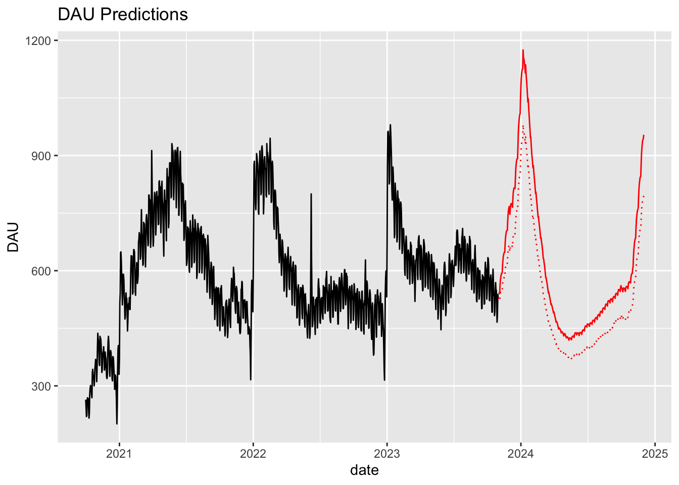
The prominent contributer to DAU counts are current users, who are aided by addition of new users everyday and the fact that current users stay active with a probability of 85% (from M matrix).
The prediction makes intuitive sense however the magnitude of spike certainly seems quite large.
Observing the shape of predicted DAU, it seems quite strongly influenced by predicted new user count from the model earlier. Additionally, some degree of experimentation with the predictions suggest that about 20% decrease in new user counts bring predicted DAU to comparable levels of previous years (dotted line in the plot).
References
Gustafson, Erin. 2024. “Meaningful Metrics: How Data Sharpened the Focus of Product Teams.” https://blog.duolingo.com/growth-model-duolingo.